
Solving The Beer Distribution Game
A data-driven approach to solving the Beer Distribution Game
Oliver Grasl
15.1.2023
The Beer Distribution Game was originally developed at MIT in the 1950s to illustrate how difficult it is to manage dynamic systems – in this case the dynamic system is a supply chain that delivers beer from a brewery to the end consumer. Play with our implementation of the Beer Distribution Game and learn about strategies to achieve the game objectives.
In this guide, we illustrate how to find a playing strategy for the Beer Distribution Game that achieves all game objectives.
We will do this for the single player game – but everything presented here also applies to the other game variants in principle.
If you’ve never played the game before, you should give it a try before reading this guide.
Note for Beer Game Facilitators
You can also use the approach outlined here in your own Beer Game Sessions - to guide players to find a “winning strategy” on their own.
We will take a data-driven approach to find a good playing strategy:
- play the game
- look at the results
- understand what is going on
- come up with an improved strategy.
- test this improved strategy in a new game
- keep repeating this process until our strategy fulfills all game objectives.
You can test the strategies we illustrate here directly in the Beer Distribution Game – but we have also created an interactive Beer Distribution Game Cheat Sheet for you to experiment with.
Quick Recap: Game Objectives
What are the game objectives?
The game objectives are listed in the rules page of the game, but we will recap them here, to make sure you know them and understand their implications.
Our top objective is to ensure that we satisfy the consumers' demand for beer. We do this by delivering beer from our inventory to the consumer.
If we don’t have enough beer in our inventory, we order the missing amount from our supplier. We remember how much beer we “owe” the consumer by putting it on our list of backorders.
From this, it follows that our backorder must be 0 by the end of the game.
But we also want to ensure that our inventory isn’t completely depleted, so our objective is to have 400 units of beer in our inventory by the end of the game.
If we subtract the size of our backorder from the size of our inventory, we arrive at a measure called the surplus:
- If the surplus is positive, this means we have been in our inventory and we don’t owe the consumer any beer.
- If the surplus is negative, this means we can’t satisfy consumers' demand for beer with the beer we have in our inventory and we owe the consumer beer.
Using the surplus we can state our first objective quite succinctly by saying that we want to achieve a surplus of 400 by the end of the game.
Our second objective is to keep our costs below 7,800 Euros.
How are the costs calculated?
The costs are equal to inventory costs plus backorder costs.
Therefore, if we reduce backorder quickly – by ordering enough beer – and keep our inventory low – by not ordering too much beer – we can keep our total costs low.
The third objective is to ensure that the overall supply chain costs stay below 29,300 Euros – to achieve this, we must ensure that our own ordering behavior doesn't lead to excess costs further up the supply chain.
Strategy 1: Following Suit
Now let's get started with our first game.
To start the beer game, we choose the single player mode, which means that we will take on the role of the retailer.
In the single player game, the other positions in the supply chain – the wholesaler, the distributor, and the brewery – are played by artificial players that follow a sensible ordering strategy.
In the first week, our customers – the end consumers – order 100 units of beer, so it makes sense for us also to order 100 units of beer.
Now the game moves into week two.
Again, the customers order 100 units of beer, and again we follow suit and order 100 units.
Now we are in week three, and this time the customers change their ordering behavior, leading to a total order of 400 units of beer.
Because we are taking a data-driven approach here, we don‘t need to overthink our ordering strategy at this stage: let’s just follow suit and also order 400 units of beer.
Again, the customers order 400 units of beer, so we'll do the same.
If you play the game more than once, you quickly realize, that the consumers always order 400 units of beer after the initial surge in the second week.
This is by design because we want to provide you with a stable, and simple, setting in which to practice playing the Beer Game.
Once you know how to play the game properly with these simple conditions, you can play under more difficult conditions, for instance by switching your position in the supply chain or by choosing advanced game presets (these features are available within the Multiplayer Game and Multigame respectively).
Let's get back to our game: As our customer always orders 400 units of beer from now on, we will too.
So let’s quickly zip through to the end of the game and see where this ordering strategy takes us.
Performance Appraisal
At the end of the game, we land in the performance appraisal.
The screenshots below are from the interactive Beer Game Cheat Sheet, which you can also view separately.
Let’s take a look at how we performed.
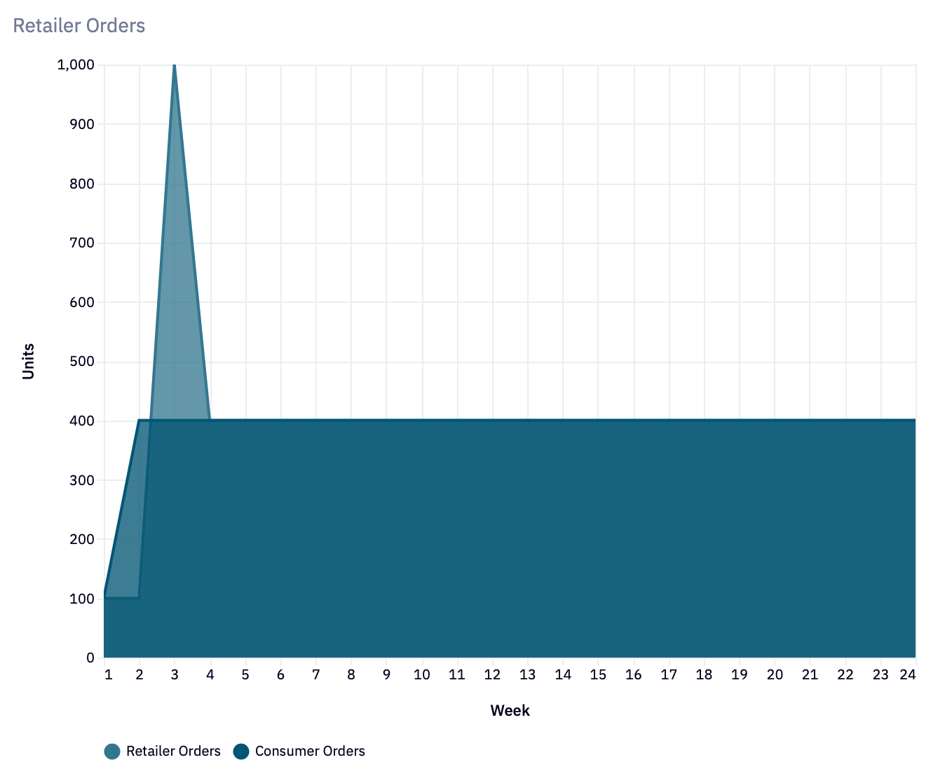
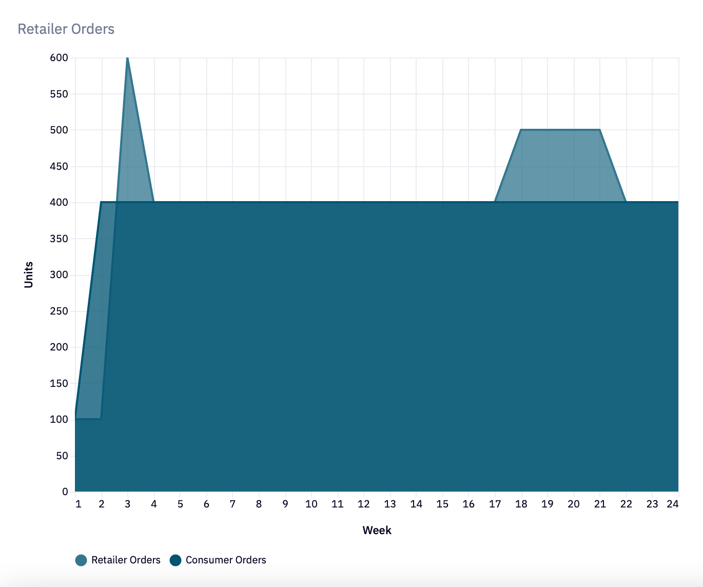
The first graph on the top left shows the order behavior of our customers and also our own response.
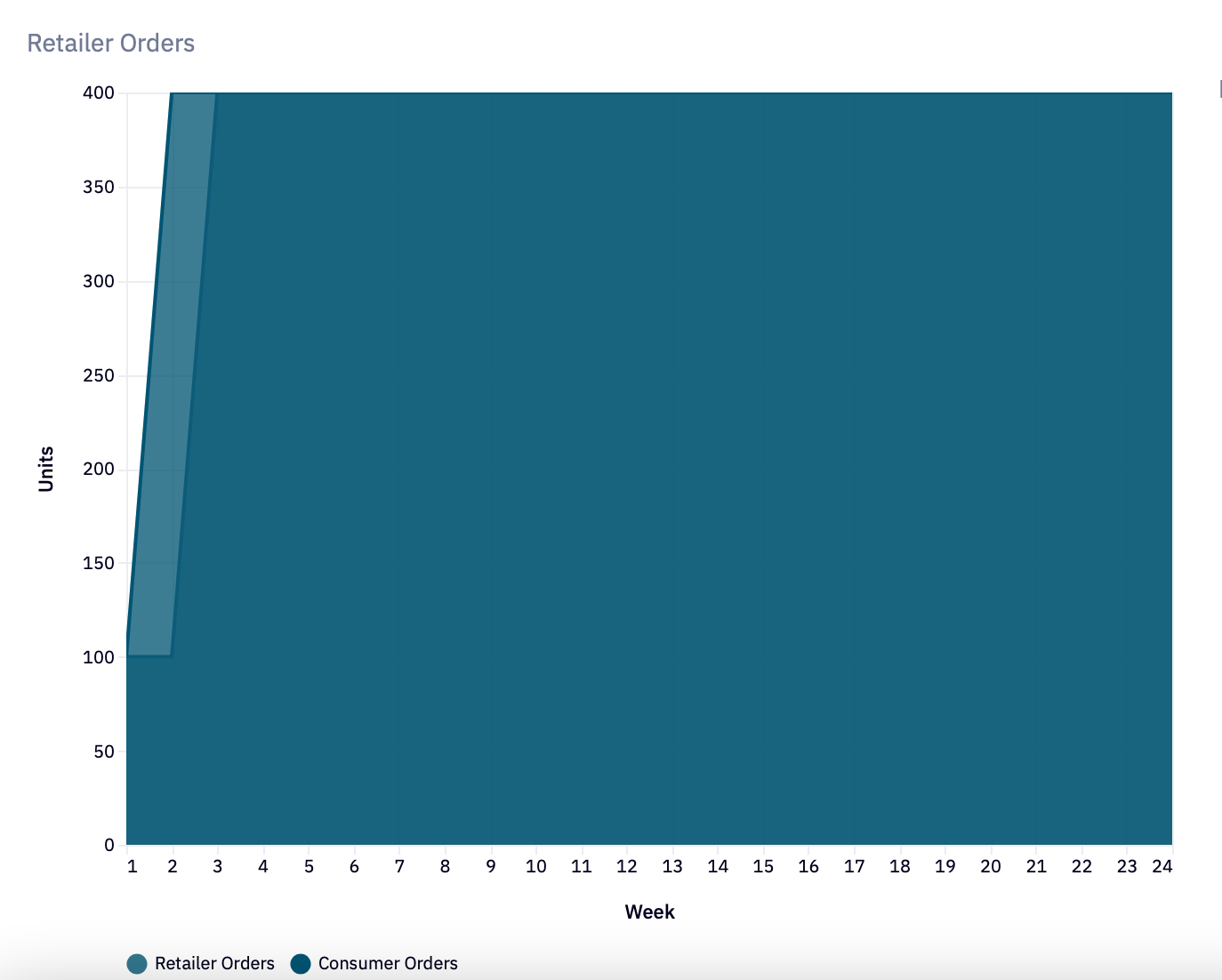
It shows that the customers ordering pattern jumped from 100 units of beer to 400 units of beer in week two.
And in response, we ordered 400 units of beer in week three and kept ordering 400 units of beer right until the end.
The next graph shows that our inventory drops from 400 units of beer down to zero units and then remains there.
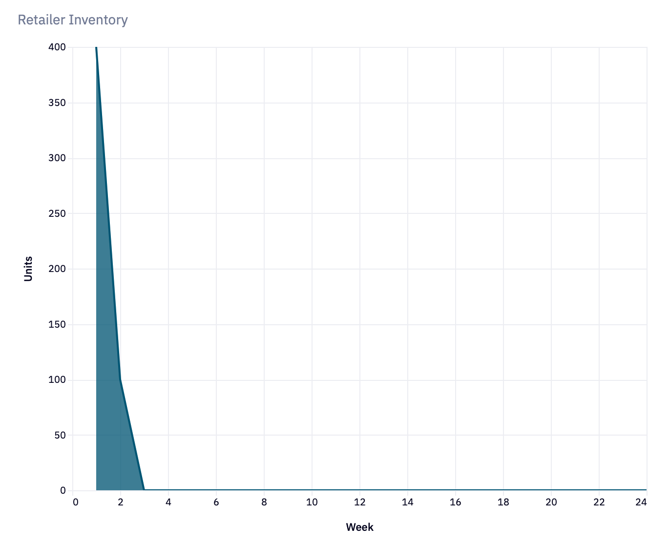
If you remember, our objective is to have an inventory of 400 units by the end of the game, so obviously we're not ordering enough beer.
But how much should we be ordering and why?
To answer this, we need to look at the backorder. The backorder rises to 800, before dropping down to 200 and remaining there.

The backorder measures the amount of beer that customers ordered but we couldn‘t deliver.
Having a backorder greater than 0 is not good at all, because if you remember what I said at the beginning of this guide, we are charged 1 Euro per round for every unit we have on backorder.
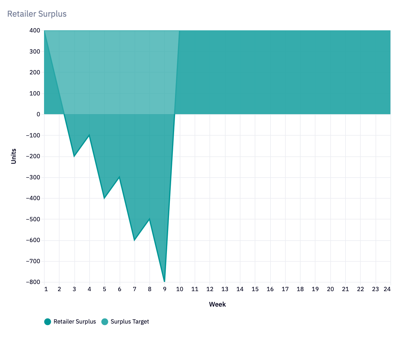
The next graph shows the surplus. We know the surplus is the difference between inventory and backorder and it thus doesn’t carry any extra information as a KPI.
But it is a very useful measure because it combines backorder and inventory into one succinct graph.
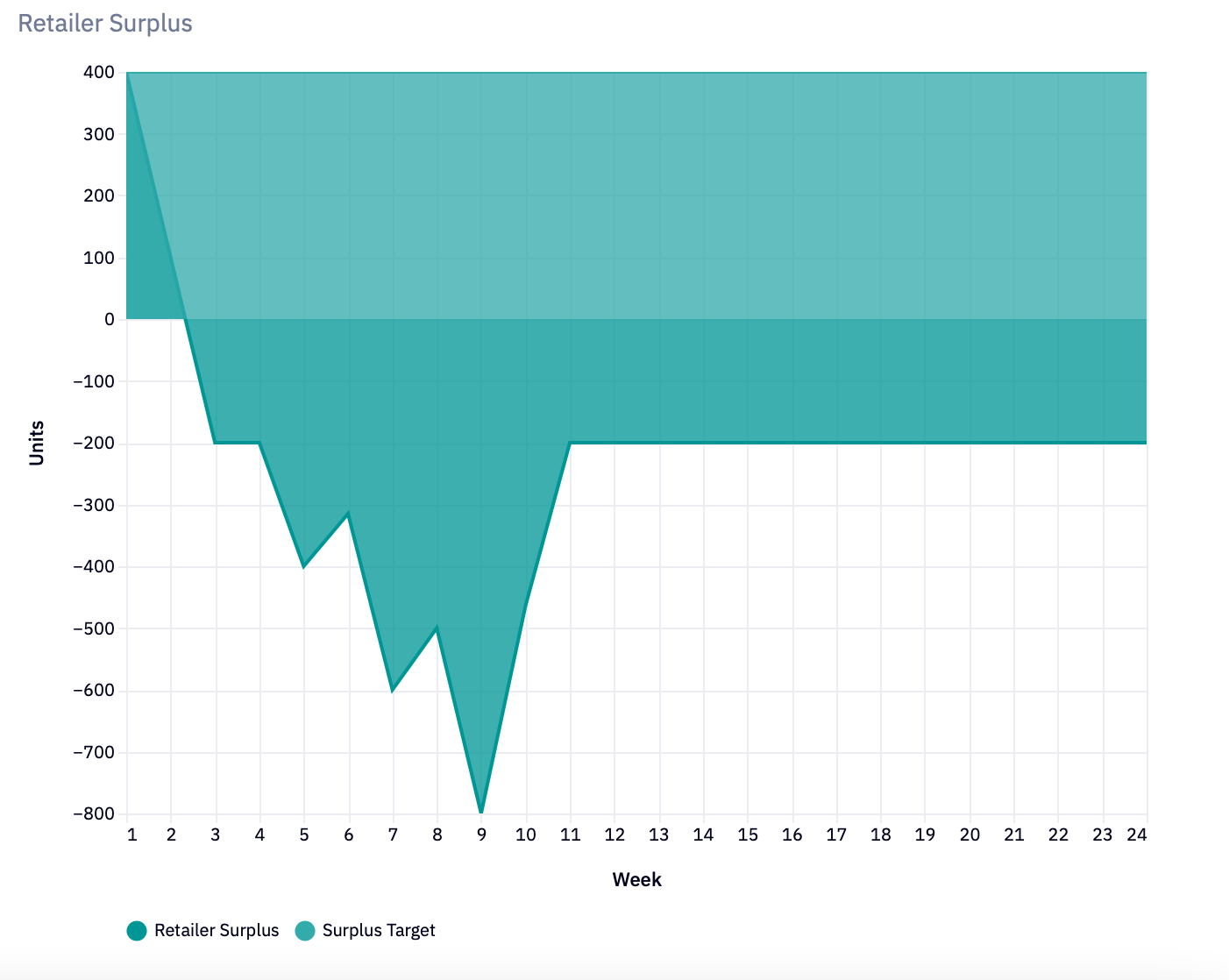
Surplus is much like a bank account: it is positive if your inventory is larger than your backorder.
It becomes negative if you owe your customers more beer than you have in stock.
In our case, the surplus is at -200. We also see the surplus target of 400 here and obviously, we have failed to reach this.
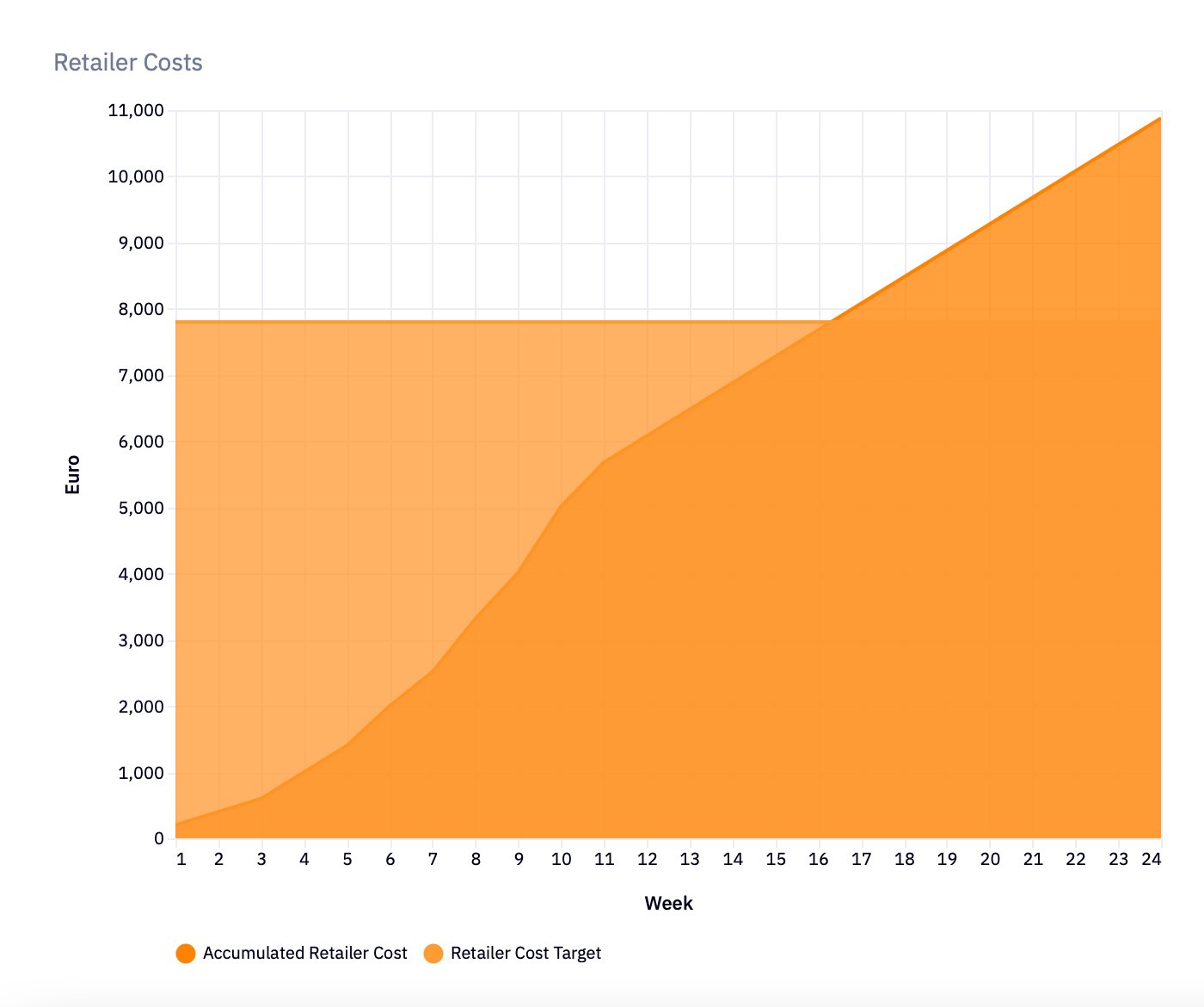
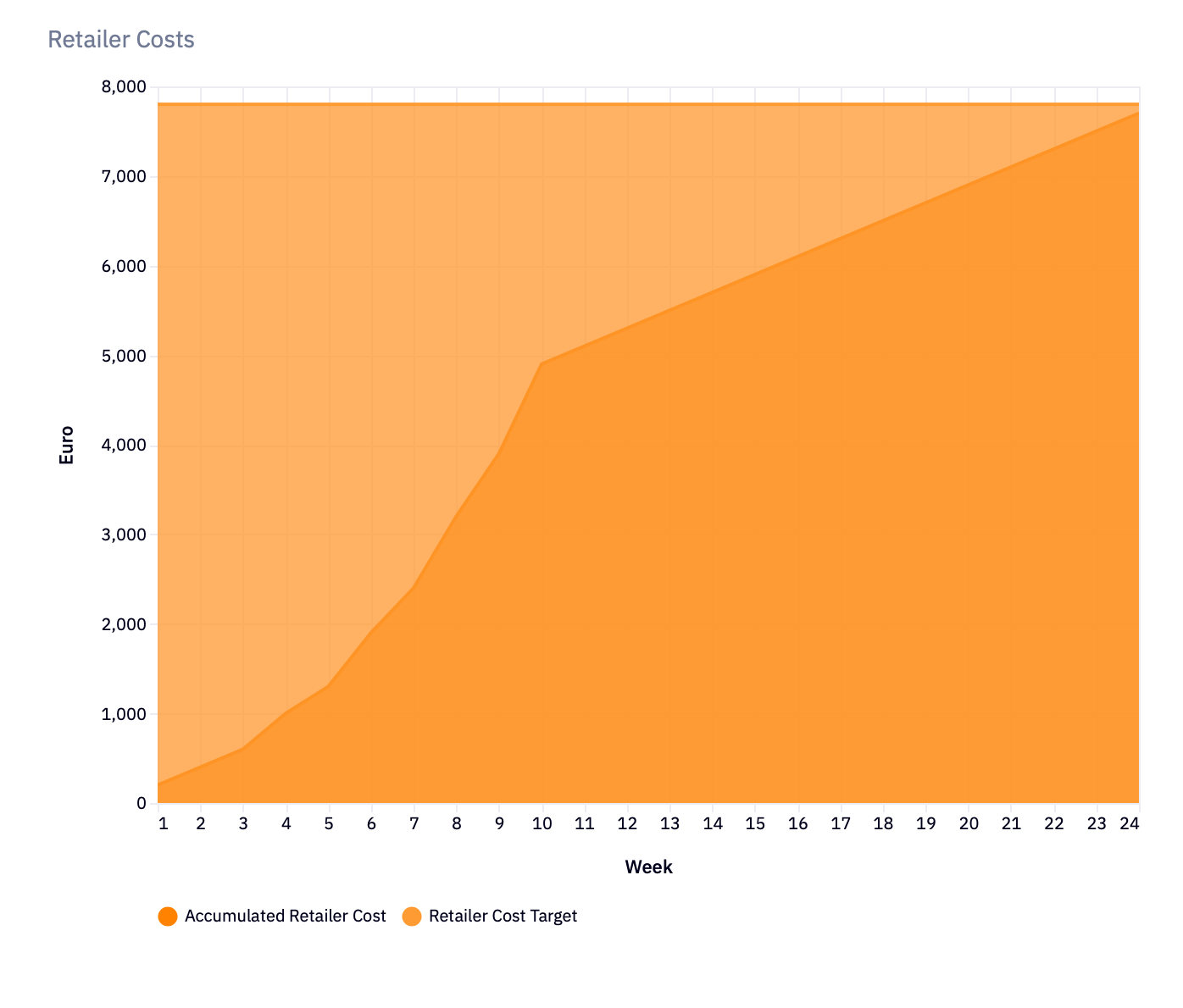
The next graph shows our costs. Our costs are way higher than the target of 7.300 Euros. This is because we were penalized in almost every round for having a backorder.
The last graph shows the overall supply chain cost.
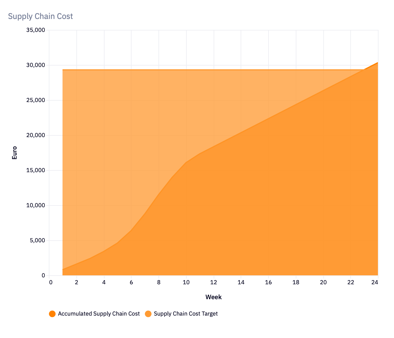
These were also higher than the target of 29.300 Euros.
They aren’t much higher though, because we avoided excessive ordering behavior and thus kept the supply chain stable.
The reason the overall costs are too high is that we failed to reach our own individual cost target.
Compensating for delays
How can we improve our ordering strategy next time around?
Clearly, we need to order those extra 200 units of beer to get our backorder to zero.
On top of that, we also need an extra 400 units to get our surplus up to the target of 400 units.
This means we need to order an extra 600 units of beer in round 3 to reach the surplus target.
Last time we ordered 400 units of beer in round three, so if we order an extra 600 units of beer, we need to order 1000 units of beer all in all.
This illustrates one of the key things about data-driven decision making: we could work out how many units of beer we need to order simply by looking at the graphs.
But there is also a danger here: we now know how much to order, but we don’t really understand where that number of 1000 units comes from.
Key Insight
There is a difference between having data and understanding that data.
So let’s think this through to get a deeper understanding of what is going on.
First of all, we need to be clear that there are some delays at work in our supply chain:
- It takes us a week to react to a change in customer orders, so we are always lagging one week behind.
- If we order beer this week, it will not arrive until next week.
- Our supplier may not have any beer in stock, so our order may arrive even later than next.
Note that the nature of these delays is different:
- the first two delays are structural delays because they are caused by the way our supply chain is set up.
- The last delay is caused by supply shortages that arise because demand is higher than the available supply.
When making an order decision, we need to account for the structural delays and ignore the delays caused by supply shortages: ordering more beer than necessary because our supplier is out of stock will only make his supply situation worse.
Hence, whenever we make an order decision, we should assume the beer will arrive in accordance with the structural delays – and if it doesn’t, due to supply shortages – we just have to sit it out.
In consequence, the order I place for week 3 not only has to account for the previous weeks order of 400, it also has to account for this weeks (anticipated) order of 400 units, so that is 800 units.
Those 800 units are only helping us to catch up though … we also anticipate receiving an order of 400 units next week, and we want to be prepared for that. So we should include 400 units for next week as well.
In total that is 3*400 units which is 1200 units of beer.
But we also must not forget that in week 2 and in week 3 we receive 100 units of beer from the wholesaler, from the orders we made in week 1 and in week 2.
1200 units of beer minus 2 times 100 units of beer equals 1000 units of beer.
Now we understand where that number of 1000 units comes from – the following table summarizes this discussion:
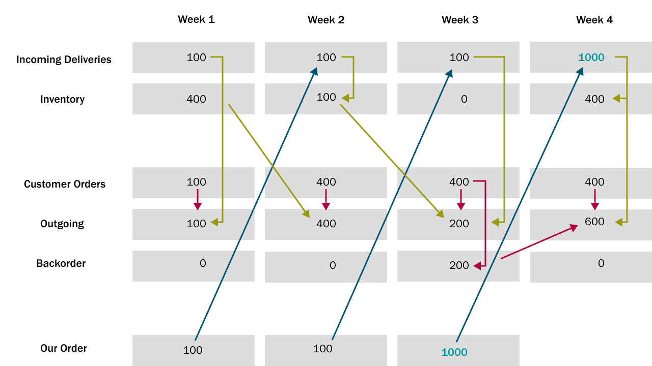
Hence our new, improved ordering strategy is to order 1000 units of beer in week 3 and then order 400 units in the following weeks.
Strategy 2: Peak Order
Please, do play the game and test the “peak order” strategy for yourself using the single player mode.
We’ll take a shortcut here though and jump right into the performance appraisal.
First, let us take a look at our ordering behavior.
In week three our customer – the consumer – ordered 400 units as expected, but here we followed our improved strategy and ordered 1000 units of beer
We can see the peak of 1000 units we ordered in week four and that our order then dropped down to 400 and remained there.
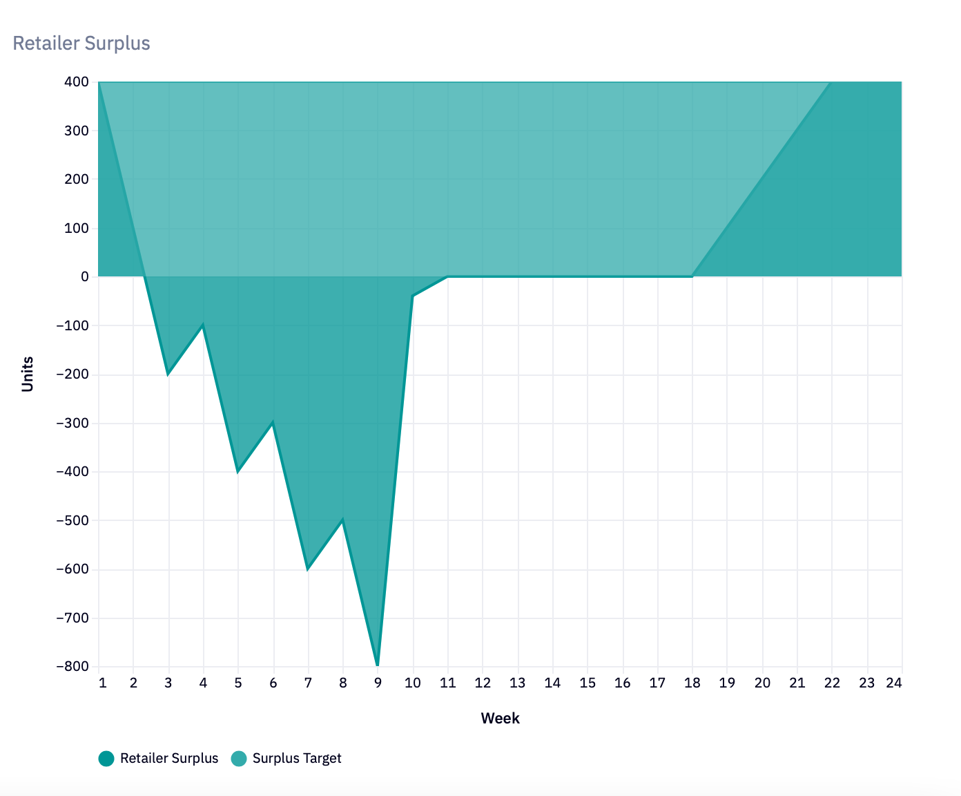
The next graph shows the surplus and we see that the surplus is at 400 by the end of the game, which is exactly what we wanted to achieve – in fact the surplus reaches 400 already in week 10.

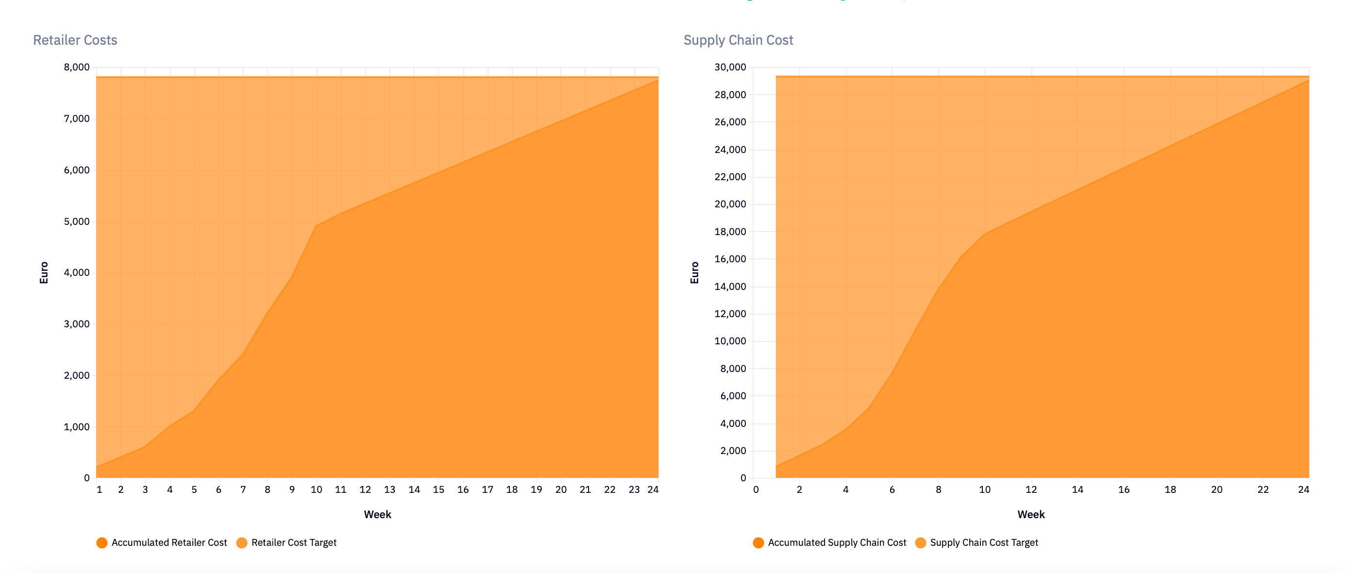
Now let's look at our costs. Our costs are actually looking very good because we reduced our backorder costs to 0 very quickly, so our costs are below our target costs and we thus have also fulfilled that objective.
Unfortunately, we can also see that our overall supply chain costs are quite a bit higher than the target supply chain cost.
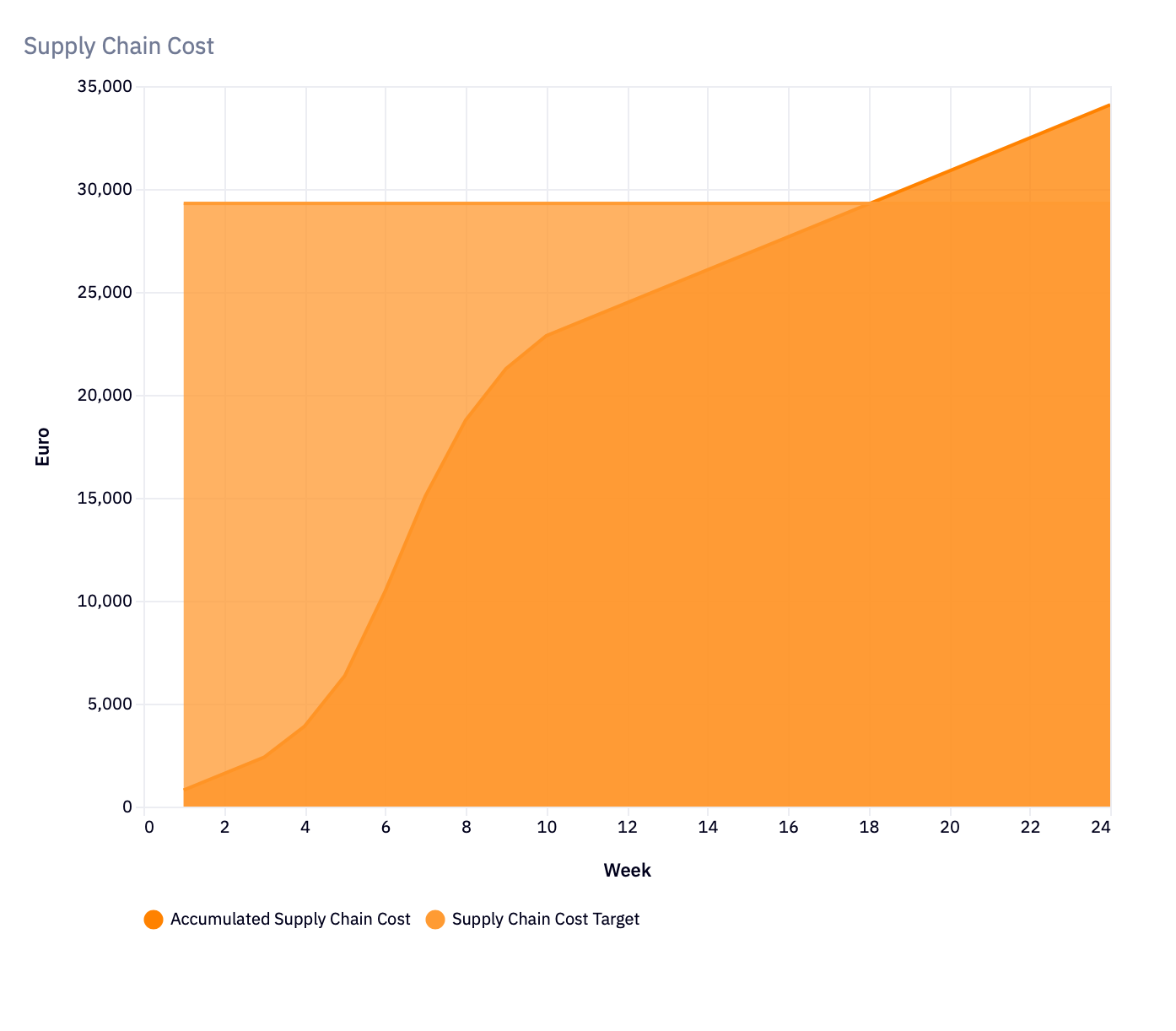
So even though we managed to reach our supply chain cost target, something in our ordering behavior must have increased the overall supply chain cost.
What exactly caused this?
The Bullwhip Effect
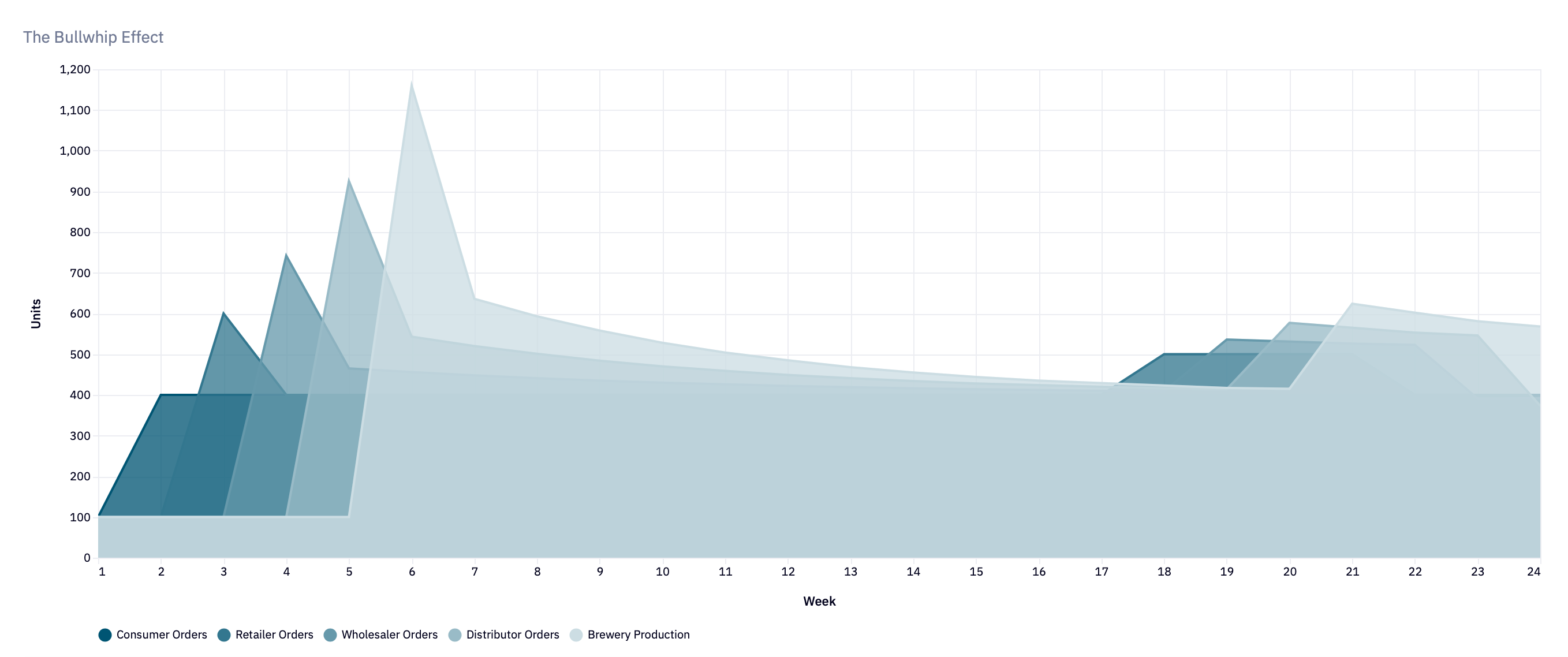
This graph compares the ordering behavior of the supply chain agents and it immediately shows what is going on:
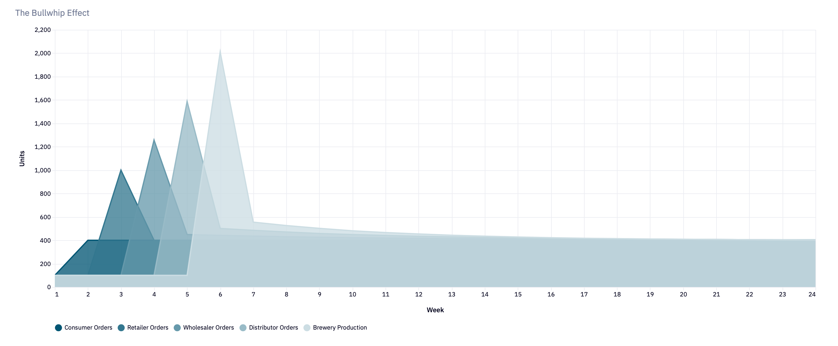
Because we order 1000 units in a week four, the next player in the supply chain – the wholesaler –is forced to order even more units of beer, 1257 ****in this case. And the distributor is forced to order even more than that – 1587 –, culminating in the brewery‘s order of 2011.
This effect is known as the bullwhip or whiplash effect: any order made at the beginning of the supply chain is amplified more and more as it travels up the supply chain.
This happens because every player in the supply chain does what we did: in order to catch up with our customers (anticipated future) demand, we order more than the customers themselves ordered.
The effect itself can only really be avoided if the entire supply chain coordinates itself in real-time. But in the Beer Game, we can only communicate via the dashboard, so all we can do is to keep the effect to a minimum by not over-ordering.
And how do we do that? How much should we order to keep our costs low, satisfy demand AND keep the bullwhip effect to a minimum?
We can answer that question by taking a closer look at our surplus. The graph shows that the surplus jumps from -800 in week 9 to plus 400 in week 10, which is exactly what we wanted.
But from the cost perspective, it would be sufficient if the surplus reaches 0 in week 10 – we would still save on the backorder cost (because backorder would be 0) and our inventory cost would remain at EUR 200 a week anyway, as long as our inventory doesn‘t rise above 400 units.
So let‘s play again, but this time we will only order 600 units in round 4. This will reduce our backorder to 0, once all the units arrive.
Then, once the supply chain has settled down, we can order the remaining 400 units we need to fill up the inventory.
But in order to keep the whiplash effect down, we won‘t order all 400 units at once – we will spread that order over four weeks, with orders of only 100 units per week.
Thus the main objective of the third strategy is to keep the peak small.
Strategy Three: Keep The Peak Small
As before we will jump right into the performance appraisal that is available in the cheat sheet.
A quick look at our ordering behavior shows that we ordered 600 units in week four. As discussed this is the minimum amount we need to order in order to get my surplus to 0.
We then consistently ordered 400 units until fairly late in the game: Starting in week 18 we order 500 units a week for 4 weeks (ie. 100 units extra) to get the surplus up to 400.
Instead of ordering the extra 400 units in bulk, we spread that order over multiple weeks on purpose, to keep the peak in the bullwhip effect small.
We can see this works nicely in the graph of the surplus: our surplus rises to 0 in week eleven and then increases steadily to 400 starting from week 18.
The order behavior comparison shows that we managed to keep the bullwhip effect to a minimum: the brewery’s peak order is now at 1200 (compared to 2011 we had in the last game). And the bullwhip effect was even smaller at the end of the game when we started filling up our inventory.
Finally, we can see here that the “Keep the Peak Small” strategy achieves all the games objectives - both our own costs and the overall costs are below the cost targets.
Great – we found a winning strategy, and it only took us three attempts!
The Golden Rule of The Beer Game
Wouldn’t it be nice if we could generalize this strategy to deal with all Beer Game Situations?
Remember that we discussed the backorder and how important it is for us to reduce our backorder to zero as quickly as possible.
But don’t forget that our supplier also has a backorder – this is the amount of beer our supplier owes us, our open orders.
Our supplier wants to get our open orders to zero as quickly as possible.
How many units of beer should we have in the open orders?
Well, think about it: We want to ensure our own backorder is 0, so our open orders should contain exactly the amount of beer we think our customers will order next week (i.e. when the beer in the open orders should arrive) plus the number of items we have on backorder (because we want to reduce the backorder, too).
Therefore, the amount of beer we order should simply be governed by our open orders and our own backorder.
Where do we see our open orders in the Beer Distribution Game?
If you check the order history (which is also available during the game), you will see column open orders: the number of units of beer we have ordered and that haven’t arrived yet.
By our reasoning above, the number of units in our open orders should always be equal to the number of orders we expect to receive from our consumers next week, plus the number of units we have on backorder.
Now let’s check the order history of the Keep The Peak Small strategy:
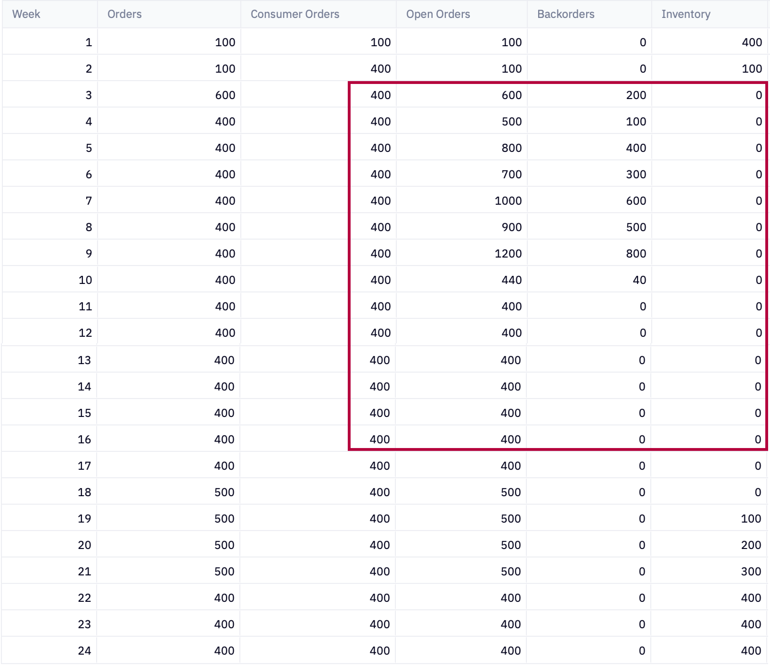
The expected order is always equal to 400 and we can see here that open orders minus backorder are always equal to 400 in weeks 2 through 16. It then rises to 500, because this is when we purposely start increasing our inventory.
Golden Rule of the Beer Distribution Game
Open Orders should always equal:
Next Week’s Expected Customer Order + Backorders
If Open Orders are larger than this, our inventory will rise (once the units of beer in the open orders arrive)
If Open Orders are smaller than this, our backorders will not go down and they may even rise
Please, do make sure you fully understand this rule and remember it well – you can apply it also to situations where the customer orders are changing, e.g. when you are playing the wholesaler, distributor, or the brewery or you are playing with advanced settings regarding consumer order behavior.
Recap
So let’s recap what we have learnt:
- We took a data-driven approach to find the right ordering strategy: we played the game, observed and interpreted the results. We came up with a better strategy, and then observed and interpreted the results again. We did this until we had found the right strategy.
- We learnt that ordering large amounts of beer can disrupt the supply chain and lead to the famous bullwhip effect.
- If the bullwhip effect is not kept in check, it causes the overall supply chain cost to rise excessively.
- The key driver of our own costs is the penalty we get for backorders. Hence the best strategy to follow in order to keep our costs down is to get backorder down to 0 as quickly as possible and then slowly increase inventory to the desired level.
- Finally, we learnt the Golden Rule of the Beer Distribution Game: the open orders should always be equal to the (anticipated) customer order plus the backorder.
- You can practice the Golden Rule in a more difficult game by playing the role of wholesaler, distributor, or brewery in a multiplayer game, or by using the advanced presets in the Multigame.

Services
Resources
All Rights Reserved.