
Sales & Operations Planning: The Planning Matters More Than The Plan
Why alignment matters more than perfect forecasts and what our interactive brewery model reveals
Sebastian Bitter, Hieu Dang
23.3.2026
No forecast is perfect and no order strategy wins every time. Companies that plan regularly are still better prepared for the unexpected. What matters is having a process that enables switching strategies when the situation changes. S&OP is an alignment process that makes trade-offs explicit before they escalate into conflicts, more than it is a forecasting tool.
1. Why Plan?
"Plans are worthless, but planning is everything." – Dwight D. Eisenhower
The general who planned the Normandy invasion knew: no plan survives first contact with the enemy. But those who do not plan get overwhelmed by that first contact.
It is no different in the supply chain. Forecasts miss the mark. Suppliers fail. Customers order differently than expected. Yesterday's plan is today's waste paper.
Yet successful companies keep planning. They know perfect forecasts are impossible. The process of planning is what prepares them for the unexpected.
That is exactly what S&OP is.
2. What is S&OP?
Sales & Operations Planning is a recurring alignment process, typically monthly, though some companies run it weekly or quarterly. The goal: Sales, Production and Finance bring their perspectives together to create a shared basis for decision-making.
The S&OP cycle in 5 steps:
Step | Phase | Who? | Key question |
1 | Data gathering | Analytics | How did we perform? |
2 | Demand planning | Sales | What demand do we expect? |
3 | Supply planning | Production | What can we deliver? |
4 | Alignment | All (incl. Finance) | What trade-offs do we accept? |
5 | Executive decision | Leadership | Decision and sign-off |

The S&OP cycle: A monthly recurring alignment process across all departments.
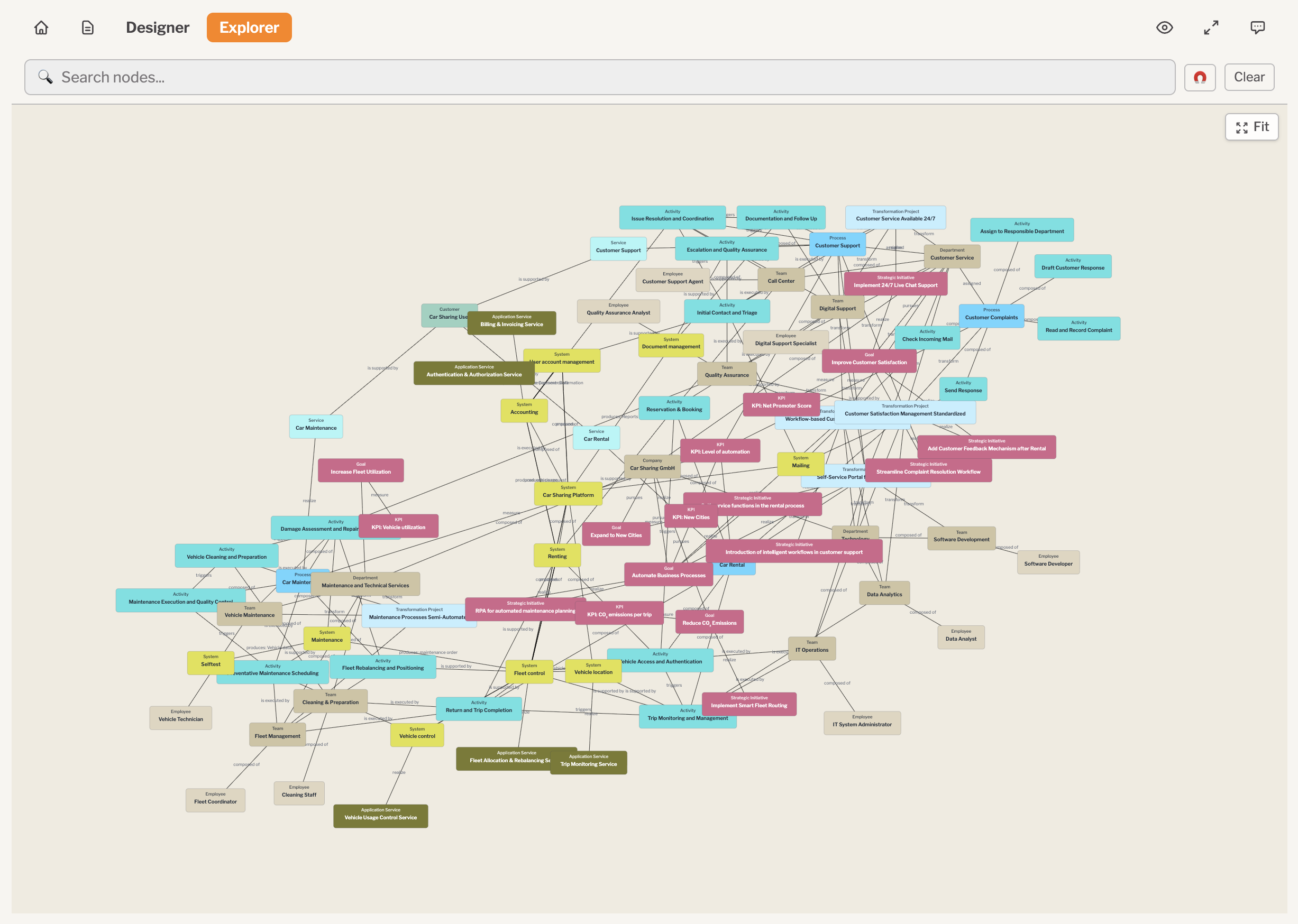
We have also formalised this process structure as a navigable metamodel in Metapad: Reviews produce Plans, Plans are measured by KPIs and Action Items lead to concrete improvements. This makes the building blocks of S&OP and their relationships explicit.
Why alignment matters so much:
Sales sees opportunities and wants availability. Production sees capacity limits and wants predictability. Finance sees tied-up capital and wants low inventory.
Without regular alignment, each function optimises for itself and the overall system loses. S&OP brings these perspectives to the table before decisions are made.
S&OP is a process for better decisions. Perfect plans are not the point.
3. ElbeBräu: An Interactive S&OP Model
To make S&OP dynamics tangible, we built an interactive digital twin in Metapad. The setting: a mid-sized brewery in Hamburg with roughly 60,000 hectolitres of annual production.
Why a brewery?
Beer combines all typical S&OP challenges in a single product. And what happens in a brewery happens everywhere: in pharmaceutical warehouses, automotive manufacturing, retail shelves. The details change, but the underlying dynamics remain the same.
The model in one picture

The complete S&OP metamodel. Seven node types (Brewery, Wholesaler, Policy Management, Controlling, Disruption, Order, Delivery) and seven relationship types describe what kinds of things can exist in the model and how they connect.
How the model works
The model is built around four monthly flows:
- NordGetränke places its monthly order.
- ElbeBräu decides what to brew, following the active order strategy (constrained by capacity and any active disruption).
- Fresh beer enters the warehouse, ages one month each tick and is delivered FIFO.
- Beer older than three months is disposed of.
Decisions take effect with a delay. Disruptions hit immediately. Too little production today is only felt two months later. A stockout today means a permanently lost customer.
How the warehouse ages
The warehouse tracks beer by age. Fresh beer arrives from the brewing pipeline, ages one month each tick and is delivered FIFO. Anything still sitting in the warehouse after three months is disposed of. You can see the cohort structure directly in one of the model's charts.

The Cohort Aging chart shows beer moving through its shelf life. Fresh beer (orange) arrives, ages one month at a time and is disposed after the third month. The interplay between production speed and demand determines how much beer makes it to disposal.
The hard constraints
Some parameters reflect typical brewery realities:
Parameter | Value | Why relevant? |
Brewing lead time | 2 months | Pilsner needs 6–8 weeks for fermentation and maturation. The decision in May determines what is in the warehouse in July. |
Shelf life | 3 months | Wholesalers will not accept beer older than 3 months. Overproduction is lost to disposal. |
Max. production capacity | 8,000 hl/month | A hard upper limit. Even the smartest forecast does not help if the kettle cannot keep up. |
Max. storage capacity | 15,000 hl | Beyond this, holding costs jump from €3/hl to €13/hl due to external warehousing. |
Seasonal swing | ~2.7× | July demand reaches 8,000 hl, January demand sits at 3,000 hl under the Seasonal scenario. |
The three levers you can play with
Three settings define each scenario:
- Demand scenario: how does the market behave? Six options from Steady to Crash.
- Order strategy: how does the brewery decide what to brew? Five strategies from naive Constant to predictive ForecastBased.
- Disruption: what goes wrong in the world? Six failure modes hitting three different parts of the supply chain (production, delivery, or shelf life).
Plus two forecast-quality dials: Forecast Bias and Forecast Error let you test what happens when the brewery's view of the future is systematically off or randomly noisy.
How success is measured
The model tracks the four KPIs that matter at year-end:
KPI | What it measures |
Service Level | Share of NordGetränke's orders that get fulfilled |
Working Capital | Cash tied up in inventory at month-end |
Stockouts | Unfulfilled demand, costs €100/hl |
Disposal | Expired product, costs €50/hl |
On top of that, the financial bottom line: revenue minus production, holding, stockout and disposal costs equals profit.
The core S&OP question
How much should the brewery brew when demand fluctuates, the forecast is uncertain and every decision only takes effect two months later?

The Sandbox view in the Metapad model shows nine charts at once: inventory and demand, monthly costs, cumulative outcome, the brewing pipeline, cohort aging, service level and the monthly P&L. Every chart recalculates instantly when you move a slider.
4. The Five Order Strategies
The model compares five order strategies, from simple to forward-looking:
1. Constant (Baseline)
Brew the same amount every month, no matter what.
The simplest possible rule. Set the production slider once and forget it. Only works well with stable demand. With seasonality: stockouts in summer, excess inventory in winter.
2. Replenishment (Reactive)
Brew exactly what came in as an order last month.
The classic ERP approach. Simple, but always one step behind. Fatal with seasonal demand: in May you brew what was needed in April, but by July demand has doubled and you are empty.
3. SeasonalNaive (Historical)
Brew today what will be needed two months from now, based on last year's seasonal pattern.
Captures seasonality as long as the pattern repeats. The two-month lookahead matches the brewing time, so the beer arrives just when demand peaks. Strong in stable seasonal worlds, but it cannot react to structural changes. If the market crashes or grows, SeasonalNaive keeps planning for last year's curve.
4. TargetInventory (Stock-aware)
Order up to a target stock level, factoring in safety stock and what is already in the brewing pipeline.
A classic base-stock policy: it asks "what do I want to have and what do I already have on hand or in transit?" Avoids double-ordering and responds flexibly to disruptions. With structural market shifts, it adapts the following year.
5. ForecastBased (Predictive)
Build a forecast of demand for the next four months and brew to a base stock target, adjusted by forecast quality.
The only forward-looking strategy. Uses the seasonal pattern as the forecast base, then applies a Bias (systematic over- or under-estimate) and Error (random month-to-month noise). The price of looking ahead: the quality of the result depends on the quality of the forecast. With +25% bias, the brewery systematically overstocks. With high error, production zigzags.
Four of the five strategies are reactive. They look at the past or at the current warehouse state and decide. Only ForecastBased is predictive, building an explicit view of the next four months. This single difference makes ForecastBased smoother in seasonal worlds, but also more sensitive to forecast quality.
5. What the Model Reveals
The model is not a calculator that hands you the right answer. It is a playground that makes the trade-offs visible. The clearest way to see those trade-offs is to run all five strategies in parallel under different world conditions and watch who survives best.
We tested five worlds. Each is a different combination of demand, disruption and forecast quality. The results show that no single strategy wins everywhere. The reason is always the same: each strategy makes different assumptions about the world and when those assumptions break, the strategy breaks with them.
World 1: Calm Year, where predictive strategies shine
Seasonal demand, no disruption, no forecast error.
Strategy | Cumulative Profit (24 months) |
Constant | 8.5M EUR |
Replenishment | 7.5M EUR |
SeasonalNaive | 9.0M EUR |
TargetInventory | 8.5M EUR |
ForecastBased | 9.5M EUR |
When the world is predictable, the forward-looking strategies (SeasonalNaive, ForecastBased) come out on top. ForecastBased uses the seasonal pattern plus a forward-looking buffer. SeasonalNaive uses the seasonal pattern without the buffer. Both anticipate the summer peaks. Replenishment chases yesterday and stays a month behind. TargetInventory and Constant land in the middle.
World 2: Demand Crash, where reactive strategies survive
The market collapses partway through the year. Production capacity reduced. Some customer churn from the resulting stockouts.
Strategy | Cumulative Profit (24 months) |
Constant | 1.9M EUR |
Replenishment | 3.7M EUR |
SeasonalNaive | 0.0M EUR |
TargetInventory | 3.3M EUR |
ForecastBased | 2.2M EUR |
The picture flips. Replenishment reacts directly to the dropping demand. TargetInventory tracks the falling orders too. SeasonalNaive collapses because it keeps ordering against last year's seasonal pattern, which does not exist anymore in a crashed market. ForecastBased has the same problem: a forecast based on the wrong world is worse than no forecast.

Demand Crash scenario. Replenishment (sand) and TargetInventory (petrol) hold their ground while SeasonalNaive (light petrol) collapses to nearly zero profit.
World 3: Saved by Bias, when a "bad" forecast becomes a hedge
Seasonal demand, MaterialShortage disruption (April to June, production stops). ForecastBased running with +30% bias and 50% error.
Strategy | Cumulative Profit (24 months) |
Constant | 5.5M EUR |
Replenishment | 6.0M EUR |
SeasonalNaive | 5.0M EUR |
TargetInventory | 4.5M EUR |
ForecastBased | 7.0M EUR |
This one is uncomfortable. A "bad" forecast (+30% bias, noisy) looks like a planning mistake under calm conditions. But the systematic over-ordering builds up safety stock that exactly fits the three-month production gap. The other strategies, including SeasonalNaive, get hit harder because they were lean.

Saved by Bias scenario. ForecastBased (orange) pulls clearly ahead because the +30% bias accidentally builds the buffer that the MaterialShortage demands.
Not every bias is a mistake. Sometimes a conservative forecast is insurance you only collect when you need it.
World 4: Perfect Storm, where robust simplicity wins
Multi-stress: DoublePeak demand, HopShortage disruption, customer churn, negative forecast bias, high error.
Strategy | Cumulative Profit (24 months) |
Constant | 6.0M EUR |
Replenishment | 6.5M EUR |
SeasonalNaive | 8.0M EUR |
TargetInventory | 6.5M EUR |
ForecastBased | 6.0M EUR |
Everything wrong at once. The smart strategies stop being smart. ForecastBased is biased the wrong way and noisy at the same time. TargetInventory gets blindsided by the unexpected second demand peak. SeasonalNaive wins by quietly following the seasonal curve through the chaos. Robust beats clever.
World 5: Stable Disruption, where TargetInventory takes the lead
Steady demand, but a MaterialShortage hits in spring. TargetInventory runs with a lead-time-aware target.
Strategy | Cumulative Profit (24 months) |
Constant | 6.5M EUR |
Replenishment | 7.0M EUR |
SeasonalNaive | 5.5M EUR |
TargetInventory | 7.5M EUR |
ForecastBased | 7.5M EUR |
The world TargetInventory was designed for: steady demand with occasional shocks. The order-up-to logic builds buffer steadily and the buffer absorbs the disruption when it comes. ForecastBased lands on the same level through its own buffer mechanism. SeasonalNaive overproduces because it expects seasonal swings that are not there in a steady market.
The lesson across five worlds
Five worlds, four different winning strategies:
World | Winner |
Calm Year | ForecastBased ≈ SeasonalNaive |
Demand Crash | Replenishment |
Saved by Bias | ForecastBased |
Perfect Storm | SeasonalNaive |
Stable Disruption | TargetInventory ≈ ForecastBased |
The implication for real S&OP: you cannot pick one strategy and forget about it. A regular planning rhythm that revisits the choice based on the current market, the current forecast quality and the current operational reality is worth more than any single algorithm.
The method matters less than the quality of alignment. Which strategy fits depends on what you know about the market, forecast quality and your own risk tolerance. S&OP brings these puzzle pieces together.
Try the comparison yourself
In the Metapad model, the Strategy Comparison view runs all five strategies in parallel under shared conditions. Use the parameter set dropdown to switch between the five worlds above, or build your own by moving the sliders. The model recalculates instantly.
6. What This Means for Your S&OP Process
S&OP is more than forecasting. A good forecast matters, but it is only one building block. S&OP delivers value even without a perfect forecast: it forces alignment, makes assumptions debatable and creates a framework for trade-offs.
Not all bias is equal. Overestimation can help during disruptions (more buffer against stockouts), but it is no free pass: higher holding costs, tied-up capital and with perishable goods, more disposal. Regular comparison of forecast vs. actuals shows which direction the deviation goes and whether it fits the cost structure.
Trade-offs do not disappear. Sales wants availability, Finance wants low inventory. The value of S&OP lies in making this tension explicit before it turns into conflict.
Communication beats methodology. No single department can choose the right strategy alone. The choice depends on forecast quality, market stability and risk tolerance. These questions can only be answered together.
The best method matters less than how well the company communicates.
7. Try It Yourself
The model runs live in your browser. Three settings define each scenario:
- Demand scenario: how does the market develop?
- Order strategy: how does the brewery respond?
- Disruption: what goes wrong?
After every change, the charts update automatically. The KPIs at the top show service level, inventory, stockouts and profit.
Three experiments to get started:
Experiment 1: Reactive vs. Forward-looking Scenario Seasonal, no disruption. Compare Replenishment with TargetInventory. Watch the summer months: Replenishment lags behind every peak, TargetInventory anticipates it. Same world, very different inventory curves.
Experiment 2: The price of forecasting Scenario Seasonal, strategy ForecastBased. Set Bias to −20%. Then switch to TargetInventory with the same scenario. TargetInventory stays stable, ForecastBased collapses, because a biased forecast acts on every month, while TargetInventory just reads the warehouse.
Experiment 3: Random vs. systematic deviation Strategy ForecastBased, Scenario Seasonal. Compare Bias=0%, Error=50 with Bias=−10%, Error=0. The random error averages out, the bias accumulates. Two very different stories with very similar numbers.
Or see all five strategies at once. Open the Strategy Comparison view in the model. It runs all five strategies in parallel under the same conditions, so you can compare them directly without switching back and forth. The parameter set dropdown gives you quick access to the five worlds from Section 5, or you can build your own.
8. What is Next?
This article has shown: neither the perfect forecast nor the cleverest order method guarantees success. What counts is cross-functional alignment between Sales, Production and Finance: the core of S&OP.
In the next article, we move from theory to disruption: When the Plan Falls Apart. What happens when a supplier fails or logistics grind to a halt? And why S&OP makes the difference between surviving a disruption and being overwhelmed by it.
The core question: the disruption itself matters less than whether there is a process behind it.
Want to experience supply chain dynamics first-hand? In the Beergame you take on a role in the supply chain and experience the bullwhip effect for yourself.
Want to explore the structure behind S&OP? In our S&OP Process Model on Metapad you can navigate the metamodel from Data Review to Executive S&OP and see how Reviews, Plans, KPIs and Action Items connect. Learn more about Metapad.


Resources
All Rights Reserved.